
To Represent the Gradient of Scalar Field and Divergence and Curl of Vector Field using Scilab
1. Aim
To visualize and understand the concepts of gradient of scalar fields, Divergence, and curl of vector fields using Scilab computational tools.
2. Apparatus Used
- Computer with Scilab installed (Version 6.0 or later recommended)
- Scilab documentation for plotting and vector field operations
- Mathematical equations and test cases prepared for demonstration
- Projection device (optional, for demonstration purposes)
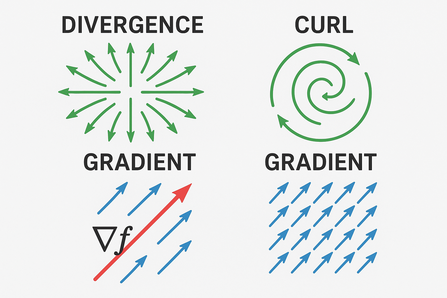
3. Diagram
Below are the sample diagrams representing vector fields and scalar fields:
4. Theory
Vector calculus is a branch of mathematics that studies differentiation and integration of vector fields. It provides the mathematical framework for modeling various physical phenomena such as fluid dynamics, electromagnetism, and thermodynamics.
Scalar Field
A scalar field assigns a scalar value to each point in space. Examples include temperature distribution, pressure field, and electric potential.
Vector Field
A vector field assigns a vector to each point in space. Examples include velocity field in fluid flow, electric field, and magnetic field.
Gradient of a Scalar Field
The gradient of a scalar field is a vector field whose magnitude represents the maximum rate of change of the scalar field, and its direction is the direction of maximum increase.
Divergence of a Vector Field
The divergence of a vector field measures the net flow of the field through a small region around each point. A positive divergence indicates a source, while a negative divergence indicates a sink.
Curl of a Vector Field
The curl of a vector field measures the field's tendency to rotate around a point. It is a vector quantity whose direction represents the axis of rotation according to the right-hand rule.
Physical Interpretation
- Gradient: Points in the direction of steepest ascent of a scalar field
- Divergence: Represents sources or sinks in a vector field (like fluid flow or electric field)
- Curl: Represents rotational behavior in a vector field (like fluid vortices or magnetic fields)
5. Formulas
Gradient of a Scalar Field
For a scalar field $f(x,y,z)$, the gradient is defined as:
$$\nabla f = \frac{\partial f}{\partial x}\hat{i} + \frac{\partial f}{\partial y}\hat{j} + \frac{\partial f}{\partial z}\hat{k}$$Divergence of a Vector Field
For a vector field $\vec{F} = F_1\hat{i} + F_2\hat{j} + F_3\hat{k}$, the divergence is defined as:
$$\nabla \cdot \vec{F} = \frac{\partial F_1}{\partial x} + \frac{\partial F_2}{\partial y} + \frac{\partial F_3}{\partial z}$$Curl of a Vector Field
For a vector field $\vec{F} = F_1\hat{i} + F_2\hat{j} + F_3\hat{k}$, the curl is defined as:
$$\nabla \times \vec{F} = \begin{vmatrix} \hat{i} & \hat{j} & \hat{k} \\ \frac{\partial}{\partial x} & \frac{\partial}{\partial y} & \frac{\partial}{\partial z} \\ F_1 & F_2 & F_3 \end{vmatrix}$$ $$= \left(\frac{\partial F_3}{\partial y} - \frac{\partial F_2}{\partial z}\right)\hat{i} + \left(\frac{\partial F_1}{\partial z} - \frac{\partial F_3}{\partial x}\right)\hat{j} + \left(\frac{\partial F_2}{\partial x} - \frac{\partial F_1}{\partial y}\right)\hat{k}$$6. Procedure
- Setup:
- Launch Scilab on your computer
- Create a new script file (.sce extension)
- Define the Domain:
- Create a mesh grid for the domain of interest (usually 2D or 3D)
- Example code for creating a 2D mesh grid:
// Create a mesh grid
x = linspace(-5, 5, 50);
y = linspace(-5, 5, 50);
[X, Y] = meshgrid(x, y);
- Define a Scalar Field:
- Choose a scalar function to analyze (e.g., $f(x,y) = x^2 + y^2$)
- Example code:
// Define a scalar field
Z = X.^2 + Y.^2; // Example scalar field: f(x,y) = x² + y²
- Calculate the Gradient:
- Compute the partial derivatives to find the gradient
- Example code:
// Calculate gradient components using numerical differentiation
[dZdx, dZdy] = gradient(Z, x, y);
- Visualize the Scalar Field and its Gradient:
- Plot the scalar field as a surface plot
- Overlay gradient vectors on a contour plot
- Example code:
// Plot scalar field as a surface
figure(1);
surf(X, Y, Z);
title('Scalar Field f(x,y) = x² + y²');
xlabel('x'); ylabel('y'); zlabel('f(x,y)');

// Plot gradient vectors on contour plot
figure(2);
contour(X, Y, Z, 20);
hold on;
xq = X(1:3:$, 1:3:$);
yq = Y(1:3:$, 1:3:$);
u = dZdx(1:3:$, 1:3:$);
v = dZdy(1:3:$, 1:3:$);
champ(xq, yq, u, v);
title('Gradient of Scalar Field ∇f');
xlabel('x'); ylabel('y');
- Define a Vector Field:
- Choose a vector field to analyze (e.g., $\vec{F}(x,y) = (y, -x)$)
- Example code:
// Define a vector field
Fx = Y; // Example vector field: F(x,y) = (y, -x)
Fy = -X;
- Calculate the Divergence:
- Compute the partial derivatives and sum them to find the divergence
- Example code:
// Calculate divergence
[dFxdx, temp] = gradient(Fx, x, y);
[temp, dFydy] = gradient(Fy, x, y);
div = dFxdx + dFydy;
- Calculate the Curl (for 2D vector field):
- Compute the z-component of the curl for a 2D field
- Example code:
// Calculate curl (z-component for 2D fields)
[dFxdy, temp] = gradient(Fx, y, x);
[temp, dFydx] = gradient(Fy, y, x);
curl_z = dFydx - dFxdy;
- Visualize the Vector Field, Divergence, and Curl:
- Plot the vector field using arrows
- Visualize divergence and curl using color maps
- Example code:
// Plot vector field
figure(3);
xq = X(1:3:$, 1:3:$);
yq = Y(1:3:$, 1:3:$);
u = Fx(1:3:$, 1:3:$);
v = Fy(1:3:$, 1:3:$);
champ(xq, yq, u, v);
title('Vector Field F(x,y) = (y, -x)');
xlabel('x'); ylabel('y');

// Plot divergence
figure(4);
surf(X, Y, div);
title('Divergence of Vector Field (∇·F)');
xlabel('x'); ylabel('y'); zlabel('∇·F');

// Plot curl (z-component)
figure(5);
surf(X, Y, curl_z);
title('Curl of Vector Field (z-component) (∇×F)_z');
xlabel('x'); ylabel('y'); zlabel('(∇×F)_z');
- Analysis:
- Interpret the results by analyzing the plots
- Verify the calculated values with theoretical expectations
- Save Results:
- Export the plots as image files
- Save the script file for future reference
7. Observation Table
| Field Type | Function Equation | Theoretical Result | Scilab Result | Visualization |
|---|---|---|---|---|
| Scalar Field 1 | $f(x,y) = x^2 + y^2$ | $\nabla f = (2x, 2y)$ | ||
| Scalar Field 2 | $f(x,y) = \sin(x) \cdot \cos(y)$ | $\nabla f = (\cos(x)\cos(y), -\sin(x)\sin(y))$ | ||
| Vector Field 1 | $\vec{F}(x,y) = (y, -x)$ | $\nabla \cdot \vec{F} = 0$ $\nabla \times \vec{F} = -2\hat{k}$ |
||
| Vector Field 2 | $\vec{F}(x,y) = (x, y)$ | $\nabla \cdot \vec{F} = 2$ $\nabla \times \vec{F} = 0$ |
||
| Vector Field 3 | $\vec{F}(x,y,z) = (x^2, y^2, z^2)$ | $\nabla \cdot \vec{F} = 2x + 2y + 2z$ $\nabla \times \vec{F} = (0, 0, 0)$ |
8. Calculations
Here are calculations for some example fields:
Example 1: Scalar Field $f(x,y) = x^2 + y^2$
To find the gradient:
$$\nabla f = \frac{\partial f}{\partial x}\hat{i} + \frac{\partial f}{\partial y}\hat{j}$$ $$\frac{\partial f}{\partial x} = \frac{\partial}{\partial x}(x^2 + y^2) = 2x$$ $$\frac{\partial f}{\partial y} = \frac{\partial}{\partial y}(x^2 + y^2) = 2y$$ $$\therefore \nabla f = 2x\hat{i} + 2y\hat{j}$$Example 2: Vector Field $\vec{F}(x,y) = (y, -x)$
To find the divergence:
$$\nabla \cdot \vec{F} = \frac{\partial F_1}{\partial x} + \frac{\partial F_2}{\partial y}$$ $$\frac{\partial F_1}{\partial x} = \frac{\partial}{\partial x}(y) = 0$$ $$\frac{\partial F_2}{\partial y} = \frac{\partial}{\partial y}(-x) = 0$$ $$\therefore \nabla \cdot \vec{F} = 0 + 0 = 0$$To find the curl (z-component for 2D field):
$$(\nabla \times \vec{F})_z = \frac{\partial F_2}{\partial x} - \frac{\partial F_1}{\partial y}$$ $$\frac{\partial F_2}{\partial x} = \frac{\partial}{\partial x}(-x) = -1$$ $$\frac{\partial F_1}{\partial y} = \frac{\partial}{\partial y}(y) = 1$$ $$\therefore (\nabla \times \vec{F})_z = -1 - 1 = -2$$Example 3: Vector Field $\vec{F}(x,y,z) = (x^2, y^2, z^2)$
To find the divergence:
$$\nabla \cdot \vec{F} = \frac{\partial F_1}{\partial x} + \frac{\partial F_2}{\partial y} + \frac{\partial F_3}{\partial z}$$ $$\frac{\partial F_1}{\partial x} = \frac{\partial}{\partial x}(x^2) = 2x$$ $$\frac{\partial F_2}{\partial y} = \frac{\partial}{\partial y}(y^2) = 2y$$ $$\frac{\partial F_3}{\partial z} = \frac{\partial}{\partial z}(z^2) = 2z$$ $$\therefore \nabla \cdot \vec{F} = 2x + 2y + 2z$$To find the curl:
$$\nabla \times \vec{F} = \begin{vmatrix} \hat{i} & \hat{j} & \hat{k} \\ \frac{\partial}{\partial x} & \frac{\partial}{\partial y} & \frac{\partial}{\partial z} \\ x^2 & y^2 & z^2 \end{vmatrix}$$Computing each component:
$$(\nabla \times \vec{F})_x = \frac{\partial F_3}{\partial y} - \frac{\partial F_2}{\partial z} = \frac{\partial z^2}{\partial y} - \frac{\partial y^2}{\partial z} = 0 - 0 = 0$$ $$(\nabla \times \vec{F})_y = \frac{\partial F_1}{\partial z} - \frac{\partial F_3}{\partial x} = \frac{\partial x^2}{\partial z} - \frac{\partial z^2}{\partial x} = 0 - 0 = 0$$ $$(\nabla \times \vec{F})_z = \frac{\partial F_2}{\partial x} - \frac{\partial F_1}{\partial y} = \frac{\partial y^2}{\partial x} - \frac{\partial x^2}{\partial y} = 0 - 0 = 0$$ $$\therefore \nabla \times \vec{F} = (0, 0, 0)$$9. Results
From the experiments performed, we observed the following:
- The gradient of a scalar field points in the direction of steepest ascent. For example, for $f(x,y) = x^2 + y^2$, the gradient vectors point radially outward from the origin, which matches our theoretical understanding.
- The divergence of vector field $\vec{F}(x,y) = (y, -x)$ is zero everywhere, indicating that this field is incompressible (no sources or sinks).
- The curl of vector field $\vec{F}(x,y) = (y, -x)$ is constant and equal to $-2\hat{k}$, indicating uniform clockwise rotation throughout the field.
- The visualization of vector field $\vec{F}(x,y) = (x, y)$ shows outward flow from the origin, consistent with its positive divergence value of 2.
- For the vector field $\vec{F}(x,y,z) = (x^2, y^2, z^2)$, the divergence increases as we move away from the origin, and the curl is zero everywhere, confirming it is an irrotational (conservative) field.
These observations verify the fundamental principles of vector calculus and demonstrate the utility of Scilab for visualizing and calculating field properties.
10. Precautions
- Ensure that the domain is properly defined with appropriate resolution for accurate visualization.
- For complex scalar and vector fields, increase the mesh density for more accurate derivative computations.
- Be careful with the scaling of vectors when visualizing gradient and vector fields.
- When plotting multiple fields on the same figure, use appropriate scales and legends for clarity.
- Numerical differentiation may introduce errors; compare numerical results with analytical solutions when possible.
- For 3D fields, consider using slices or 2D projections to visualize the field properties effectively.
- Save workspace and script files periodically to prevent data loss.
- Verify the sign conventions used in the curl and gradient calculations.
- Check that the units are consistent throughout all calculations.
- For large datasets, optimize the code to improve performance.
11. Viva Voice Questions
1. What is the physical significance of the gradient of a scalar field?
The gradient of a scalar field represents both the direction of maximum rate of change of the field and the magnitude of that rate of change. Physically, it can represent forces in potential fields (like gravitational or electric fields), pressure gradients in fluid dynamics, or temperature gradients in heat transfer problems.
2. Why is the divergence of the vector field $\vec{F}(x,y) = (y, -x)$ equal to zero?
The divergence measures the net outflow of a vector field from a point. For $\vec{F}(x,y) = (y, -x)$, we calculate $\nabla \cdot \vec{F} = \frac{\partial F_1}{\partial x} + \frac{\partial F_2}{\partial y} = \frac{\partial y}{\partial x} + \frac{\partial (-x)}{\partial y} = 0 + 0 = 0$. This vector field represents circular motion around the origin, so there is no net outflow or inflow at any point, making the divergence zero.
3. What is the difference between a conservative and a non-conservative vector field?
A conservative vector field is one whose curl is zero everywhere, meaning it can be expressed as the gradient of a scalar potential function. In such fields, the work done in moving along any closed path is zero. Non-conservative fields have non-zero curl at some points, and work depends on the path taken. Examples of conservative fields include gravitational and electrostatic fields, while magnetic fields are non-conservative.
4. How would you determine if a given vector field is solenoidal?
A solenoidal vector field has zero divergence everywhere. To determine if a vector field $\vec{F}$ is solenoidal, we compute $\nabla \cdot \vec{F}$ and check if it equals zero throughout the domain. If the divergence is zero everywhere, the field is solenoidal, meaning it has no sources or sinks and satisfies the condition of incompressibility.
5. What are the applications of gradient, divergence, and curl in physics and engineering?
Gradient: Used in optimization problems, potential theory (electric and gravitational fields), heat transfer (temperature gradients), and fluid dynamics (pressure gradients).
Divergence: Applied in fluid dynamics (mass conservation), electromagnetism (Gauss's law), and heat transfer (heat source distribution).
Curl: Utilized in electromagnetism (Ampere's law), fluid dynamics (vorticity analysis), and mechanical engineering (rotation of stress tensors).
6. Why is numerical differentiation less accurate than analytical differentiation?
Numerical differentiation approximates derivatives using finite differences, which introduces truncation errors. These errors depend on the step size used in the approximation. Additionally, floating-point arithmetic in computers introduces round-off errors. In contrast, analytical differentiation provides exact expressions for derivatives based on mathematical rules. When implementing in Scilab, these numerical errors can affect the accuracy of gradient, divergence, and curl calculations, especially for functions with rapid variations.
7. Explain the concept of the Laplacian operator and its significance.
The Laplacian operator ($\nabla^2$ or $\Delta$) is the divergence of the gradient of a scalar field. It is defined as $\nabla^2 f = \nabla \cdot (\nabla f) = \frac{\partial^2 f}{\partial x^2} + \frac{\partial^2 f}{\partial y^2} + \frac{\partial^2 f}{\partial z^2}$ in 3D. The Laplacian is significant in many areas of physics and engineering as it appears in important differential equations like Poisson's equation and the wave equation. In physical terms, the Laplacian represents the flux density of the gradient flow of a function and is used in heat flow, diffusion processes, electrostatics, and quantum mechanics.