
Study of OP AMP as Non-Inverting Amplifier
1. Aim
To study the characteristics and behavior of an Operational Amplifier (OP AMP) configured as a non-inverting amplifier, verify its voltage gain, and analyze its performance under different input conditions.
2. Apparatus Used
- IC 741 Operational Amplifier
- DC Power Supply (±15V)
- Digital Multimeter or Oscilloscope
- Connecting Wires
- Breadboard
- Resistors (1kΩ, 10kΩ, and other values as needed)
- Function Generator (for AC signal analysis)
- Potentiometer (10kΩ)
3. Circuit Diagram
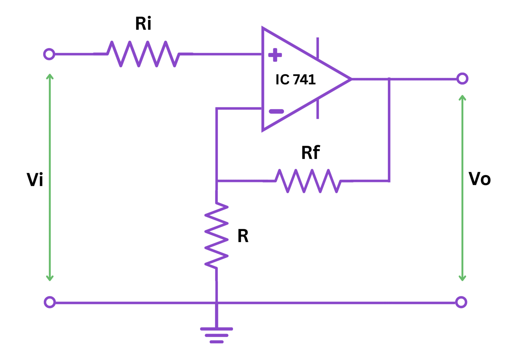
Figure 1: Circuit diagram of non-inverting amplifier using OP AMP 741
4. Theory
A non-inverting amplifier is a fundamental operational amplifier configuration that amplifies the input signal without inverting its phase. The operational amplifier (commonly IC 741) is connected with negative feedback to control the gain accurately.
The non-inverting amplifier has high input impedance, making it suitable for applications where loading effects must be minimized. The input signal is applied to the non-inverting terminal (positive input), and feedback is provided from the output to the inverting terminal (negative input) through resistors.
Two key principles are at work in this configuration:
- Virtual Short Concept: When an op-amp operates in its linear region with negative feedback, the voltage difference between its two input terminals approaches zero.
- Zero Input Current Principle: The input terminals of an ideal op-amp draw negligible current.
These principles lead to the derivation of the voltage gain equation. If we denote the input voltage as $V_{in}$ and the output voltage as $V_{out}$, the voltage gain $A_v$ of the non-inverting amplifier is given by:
Where:
- $R_f$ is the feedback resistor
- $R_1$ is the resistor connected between the inverting input and ground
The minimum gain of a non-inverting amplifier is 1 (when $R_f = 0$ or $R_1 = \infty$), unlike the inverting configuration where the gain can be less than 1.
5. Formula
Voltage Gain ($A_v$): $A_v = \frac{V_{out}}{V_{in}} = 1 + \frac{R_f}{R_1}$
Output Voltage ($V_{out}$): $V_{out} = V_{in} \times \left(1 + \frac{R_f}{R_1}\right)$
Theoretical Gain ($A_{th}$): $A_{th} = 1 + \frac{R_f}{R_1}$
Practical Gain ($A_{pr}$): $A_{pr} = \frac{V_{out}}{V_{in}}$ (measured)
Percentage Error: $\text{Error}(\%) = \frac{|A_{th} - A_{pr}|}{A_{th}} \times 100\%$
6. Procedure
- Set up the circuit on the breadboard as per the circuit diagram shown in Figure 1.
- Connect the power supply to the op-amp (±15V to pins 7 and 4 of IC 741).
- Select appropriate values for the resistors $R_1$ and $R_f$ to achieve the desired gain.
- For Trial 1: $R_1 = 1\text{ k}\Omega$, $R_f = 10\text{ k}\Omega$ (Theoretical gain = 11)
- For Trial 2: $R_1 = 2.2\text{ k}\Omega$, $R_f = 10\text{ k}\Omega$ (Theoretical gain ≈ 5.55)
- For Trial 3: $R_1 = 4.7\text{ k}\Omega$, $R_f = 10\text{ k}\Omega$ (Theoretical gain ≈ 3.13)
- For DC analysis:
- Connect a variable DC voltage source to the non-inverting input terminal.
- Vary the input voltage from 0.1V to 1.0V in steps of 0.1V.
- For each input voltage, measure the output voltage using the multimeter.
- Record all readings in the observation table.
- For AC analysis (optional):
- Connect a function generator to the non-inverting input terminal.
- Set the input to a sine wave with frequency 1kHz and amplitude 0.5V peak-to-peak.
- Observe the input and output waveforms on the oscilloscope.
- Measure the amplitudes of both waveforms and calculate the gain.
- Repeat for different frequencies (100Hz, 10kHz, 100kHz) to observe frequency response.
- Change the resistor values as per the next trial and repeat steps 4-5.
- Calculate the practical gain for each set of readings.
- Calculate the percentage error between theoretical and practical gains.
- Plot a graph of output voltage versus input voltage for each configuration.
7. Observation Table
For Trial 1: $R_1 = 1\text{ k}\Omega$, $R_f = 10\text{ k}\Omega$ (Theoretical gain = 11)
| S.No. | Input Voltage $V_{in}$ (V) | Output Voltage $V_{out}$ (V) | Practical Gain $A_{pr} = \frac{V_{out}}{V_{in}}$ |
|---|---|---|---|
| 1 | 0.1 | ||
| 2 | 0.2 | ||
| 3 | 0.3 | ||
| 4 | 0.4 | ||
| 5 | 0.5 | ||
| 6 | 0.6 | ||
| 7 | 0.7 | ||
| 8 | 0.8 | ||
| 9 | 0.9 | ||
| 10 | 1.0 |
For Trial 2: $R_1 = 2.2\text{ k}\Omega$, $R_f = 10\text{ k}\Omega$ (Theoretical gain ≈ 5.55)
| S.No. | Input Voltage $V_{in}$ (V) | Output Voltage $V_{out}$ (V) | Practical Gain $A_{pr} = \frac{V_{out}}{V_{in}}$ |
|---|---|---|---|
| 1 | 0.1 | ||
| 2 | 0.2 | ||
| 3 | 0.3 | ||
| 4 | 0.4 | ||
| 5 | 0.5 | ||
| 6 | 0.6 | ||
| 7 | 0.7 | ||
| 8 | 0.8 | ||
| 9 | 0.9 | ||
| 10 | 1.0 |
For Trial 3: $R_1 = 4.7\text{ k}\Omega$, $R_f = 10\text{ k}\Omega$ (Theoretical gain ≈ 3.13)
| S.No. | Input Voltage $V_{in}$ (V) | Output Voltage $V_{out}$ (V) | Practical Gain $A_{pr} = \frac{V_{out}}{V_{in}}$ |
|---|---|---|---|
| 1 | 0.1 | ||
| 2 | 0.2 | ||
| 3 | 0.3 | ||
| 4 | 0.4 | ||
| 5 | 0.5 | ||
| 6 | 0.6 | ||
| 7 | 0.7 | ||
| 8 | 0.8 | ||
| 9 | 0.9 | ||
| 10 | 1.0 |
8. Calculations
For each trial, perform the following calculations:
Trial 1: $R_1 = 1\text{ k}\Omega$, $R_f = 10\text{ k}\Omega$
Theoretical Gain ($A_{th}$):
Practical Gain ($A_{pr}$) for input voltage $V_{in} = 0.5\text{ V}$ (example):
Percentage Error:
Similar calculations should be performed for Trial 2 and Trial 3.
Average Practical Gain
Average Percentage Error
9. Result
Based on the observations and calculations, we can conclude:
- The non-inverting amplifier successfully amplifies the input signal without phase inversion.
- The experimental voltage gain values are compared with theoretical values:
- For Trial 1 ($R_f/R_1 = 10$): Theoretical gain = 11, Measured gain = [to be filled]
- For Trial 2 ($R_f/R_1 = 4.55$): Theoretical gain = 5.55, Measured gain = [to be filled]
- For Trial 3 ($R_f/R_1 = 2.13$): Theoretical gain = 3.13, Measured gain = [to be filled]
- The relationship between input and output voltage is linear within the operating range of the op-amp.
- The percentage error between theoretical and practical values is within an acceptable range (typically less than 5%) due to component tolerances and measurement limitations.
- The gain formula $A_v = 1 + R_f/R_1$ is experimentally verified.
10. Precautions
- Ensure proper connections and polarities of the op-amp power supply (±15V).
- Use resistors with appropriate power ratings and tolerances (preferably 1% or better).
- Avoid input signals that could lead to output saturation (beyond the supply voltage range).
- Ensure that the op-amp is operating in its linear region.
- Use proper grounding techniques to minimize noise.
- Verify the pin configuration of IC 741 before making connections.
- Allow the circuit to stabilize before taking measurements.
- Ensure the multimeter or oscilloscope is properly calibrated.
- Keep the circuit away from electromagnetic interference sources.
- Handle the IC with care to avoid damage from static electricity.
11. Viva Voice Questions
An operational amplifier (op-amp) is a high-gain voltage amplifier with differential inputs designed to amplify the voltage difference between its two input terminals. It has high input impedance, low output impedance, and typically very high open-loop gain.
In an inverting amplifier, the input signal is applied to the inverting terminal (negative input) through a resistor, causing the output to be inverted (180° phase shift). The gain formula is $A_v = -R_f/R_1$. In a non-inverting amplifier, the input signal is applied directly to the non-inverting terminal (positive input), and the output is in phase with the input. The gain formula is $A_v = 1 + R_f/R_1$.
Feedback is used to stabilize the gain, increase the bandwidth, reduce distortion, and control the input and output impedances of the amplifier. Negative feedback in particular helps make the circuit behavior more predictable and less dependent on the specific characteristics of the op-amp used.
Advantages include higher input impedance (which reduces loading effects), non-inverted output signal, minimum gain of unity (whereas inverting amplifiers have gains less than 1), and better common-mode rejection ratio in practical applications.
Virtual ground is a point in the circuit that is effectively at ground potential (0V) but is not directly connected to ground. In op-amps with negative feedback, the inverting input terminal behaves as a virtual ground when the non-inverting input is grounded, due to the very high open-loop gain that forces both inputs to be at nearly identical potentials.
The input impedance of an ideal non-inverting amplifier is infinite because the input signal is applied to the non-inverting terminal of the op-amp, which ideally draws no current.
Factors include resistor tolerances, finite open-loop gain of the op-amp, input bias currents, input offset voltages, temperature effects, frequency limitations of the op-amp, and measurement errors.
The 741 op-amp has a unity gain bandwidth of about 1 MHz, but its bandwidth decreases with increasing gain due to the gain-bandwidth product limitation.
Slew rate is the maximum rate of change of output voltage with respect to time, typically expressed in V/μs. It limits how quickly the output voltage can change in response to a step change in input. A low slew rate can cause distortion when amplifying high-frequency signals, as the op-amp cannot keep up with rapid input changes.
Common-Mode Rejection Ratio (CMRR) is a measure of an op-amp's ability to reject signals that are common to both inputs. It is important because it determines how well the op-amp can amplify differential signals while rejecting common-mode noise or interference. A higher CMRR indicates better performance in rejecting unwanted common-mode signals.